suppressPackageStartupMessages({
 library(tidymodels)
 library(tidyverse)
 library(bonsai)
 library(modeldata)
 library(mirai)
})I’ve been testing out mirai ever since I saw Charlie Gao and Will Landau’s joint talk. TLDR: it’s really good. I didn’t realize how much I needed asynchronous map functions until I had them. In this post, I’ll demo an application of mirai to speed up the tuning process for a bunch of tidymodel workflows.
Packages
We’ll load the usual tidy libraries plus bonsai (for the aorsf engine), modeldata (for the meats data), and mirai.
Data
We’ll use the meats data from the modeldata package for this post. Some details taken from ?meats are below.
These data are recorded on a Tecator Infratec Food and Feed Analyzer working in the wavelength range 850 - 1050 nm by the Near Infrared Transmission (NIT) principle. Each sample contains finely chopped pure meat with different moisture, fat and protein contents. For each meat sample the data consists of a 100 channel spectrum of absorbances and the contents of moisture (water), fat and protein. The absorbance is -log10 of the transmittance measured by the spectrometer. The three contents, measured in percent, are determined by analytic chemistry.
A special thank you to the instrument and company name (Tecator) for making these data publicly available, and a thank you to the modeldata maintainers as well.
data_meats <- modeldata::meats

data_meats
Resamples
We’ll be comparing different workflows to develop a prediction model in this post, so making a resampling object is a required step.
set.seed(321)

data_resamples <- vfold_cv(data_meats)

data_resamples
Recipe factory
The recipes package makes it so easy to compose many recipes with slightly different steps. Here, I start with a template to guide which steps to include in my recipe.
recipes_init <- tidyr::expand_grid(
 boxcox = c(TRUE, FALSE),
 pca = c(TRUE, FALSE),
 poly = c(TRUE, FALSE)
)

recipes_init
Next I go through the template line by line and make a recipe with each specification. What I like about this is the control on order and inclusion of specific steps. You can even indicate that certain steps in the recipe should be tuned, but we’ll leave that for another post.
# Generate recipes based on a grid of parameters

recipe_list <- recipes_init %>%
 mutate(
  recipe = pmap(
   .l = list(boxcox, pca, poly),
   .f = function(use_boxcox, use_pca, use_poly){

    rec_init <- recipe(protein ~ ., data = data_meats)

    if (use_boxcox) {
     rec_init <- rec_init %>%
      step_BoxCox(all_numeric_predictors())
    }

    if (use_pca) {
     rec_init <- rec_init %>%
      step_pca(all_numeric_predictors(), num_comp = 10)
    }

    if(use_poly) {
     rec_init <- rec_init %>%
      step_poly(all_numeric_predictors())
    }

    rec_init
   }
  )
 ) %>%
 mutate(
  boxcox = factor(boxcox, labels = c("box.no", "box.yes")),
  pca = factor(pca, labels = c("pca.no", "pca.yes")),
  poly = factor(poly, labels = c("poly.no", "poly.yes"))
 ) %>%
 unite(col = 'name', boxcox, pca, poly) %>%
 mutate(name = paste0(name, '.')) %>%
 deframe()

# check out the first recipe in the list

recipe_list[[1]]
── Recipe ──────────────────────────────────────────────────────────────────────── Inputs Number of variables by roleoutcome: 1
predictor: 102── Operations • Box-Cox transformation on: all_numeric_predictors()• PCA extraction with: all_numeric_predictors()• Orthogonal polynomials on: all_numeric_predictors()Model specifications
We’ll use three modeling strategies and basic tuning where we can.
model_list <- list(

   glmnet = linear_reg(penalty = tune(), mixture = tune()) %>%
    set_engine("glmnet"),

   aorsf = rand_forest(min_n = tune()) %>%
    set_engine("aorsf") %>%
    set_mode("regression"),

   svm = svm_rbf(cost = tune(),
                 rbf_sigma = tune(),
                 margin = tune()) %>%
    set_mode('regression')

  )
Workflows
We’ll start by making a data frame containing all the modeling workflows.
metrics <- metric_set(rsq, rmse)

wf <- recipe_list %>%
 workflow_set(models = model_list) %>%
 option_add(metrics = metrics)

wf
Now, how do we make wf compatible with mirai? Well, there are probably many ways to do that, but this works fine for me:
wf_split <- split(wf, f = seq(nrow(wf)))

# check out the first two workflows
wf_split[1:2]
$`1`
# A workflow set/tibble: 1 × 4
wflow_id info option result
<chr> <list> <list> <list>
1 box.yes_pca.yes_poly.yes._glmnet <tibble [1 × 4]> <opts[1]> <list [0]>
$`2`
# A workflow set/tibble: 1 × 4
wflow_id info option result
<chr> <list> <list> <list>
1 box.yes_pca.yes_poly.yes._aorsf <tibble [1 × 4]> <opts[1]> <list [0]>Why use split? Because I plan on sending each workflow object into mirai_map, which can set up asynchronous workers for each item in a list of inputs.
# tell mirai to initiate 10 workers
# (use a suitable number depending on your resources)
daemons(n = 10)

# this seems unnecessary, but bonsai's parsnip
# wrappers will only be necessary in worker's
# environments if we explicitly call library
# in the worker environments.
everywhere(library(bonsai))

# run tune_grid for each workflow, separately
res <- mirai_map(
 .x = wf_split,
 .f = workflow_map,
 .args = list(fn = 'tune_grid',
              resamples = data_resamples,
              metrics = metrics)
)
So what’s so good about asynchronous parallel programming? Well, while res is running over 10 workers, you still have access to your current R session. You can even print res and check it’s progress like so:
res< mirai map [0/24] >waits 10 seconds
res< mirai map [6/24] >waits some more
res< mirai map [24/24] >The lesson here is that mirai_map can substantially speed up how fast your code will run and also leave you free to keep working while your code runs. That’s two complementary ways to speed up your work. When all the tasks are done, put results back together like so:
# put all the workflows back together.
wf_done <- map_dfr(res, 'data')

wf_done
Visualize
Now that we’ve covered computing, let’s talk science. We tuned and evaluated three learners paired with eight unique pre-processing recipes. Let’s put together a visual to illustrate how the prediction accuracy of learners varied over these recipes.
data_gg <- wf_done %>%
   rank_results("rsq", select_best = TRUE) %>%
   filter(.metric == "rsq") %>%
   separate(col = wflow_id,
            into = c(".preproc", ".model"),
            sep = '\\.\\_',
            remove = FALSE)

data_gg <- data_gg %>%
 arrange(.preproc, desc(rank)) %>%
 mutate(text = NA_character_) %>%
 split(.$.preproc) %>%
 map2_dfr(names(.), ~add_row(.x, text = .y, .before = 1)) %>%
 mutate(x = rev(seq(n())))

top_score <- max(data_gg$mean, na.rm = TRUE)

fig <- ggplot(data_gg, aes(x = x,
                           y = mean,
                           ymin = mean - 1.96 * std_err,
                           ymax = mean + 1.96 * std_err,
                           fill = .preproc)) +
 geom_col(show.legend = FALSE) +
 coord_flip() +
 geom_text(aes(label = .model, y = mean, hjust = -0.1)) +
 geom_text(aes(label = text, y = 0, hjust = 0)) +
 geom_hline(yintercept = top_score,
            color = 'grey',
            linetype = 2) +
 theme_minimal() +
 scale_fill_viridis_d() +
 theme(axis.text.y = element_blank(),
       panel.grid = element_blank(),
       axis.line.x = element_line()) +
 labs(y = "R-squared",
      x = "",
      fill = "Pre-processing")

fig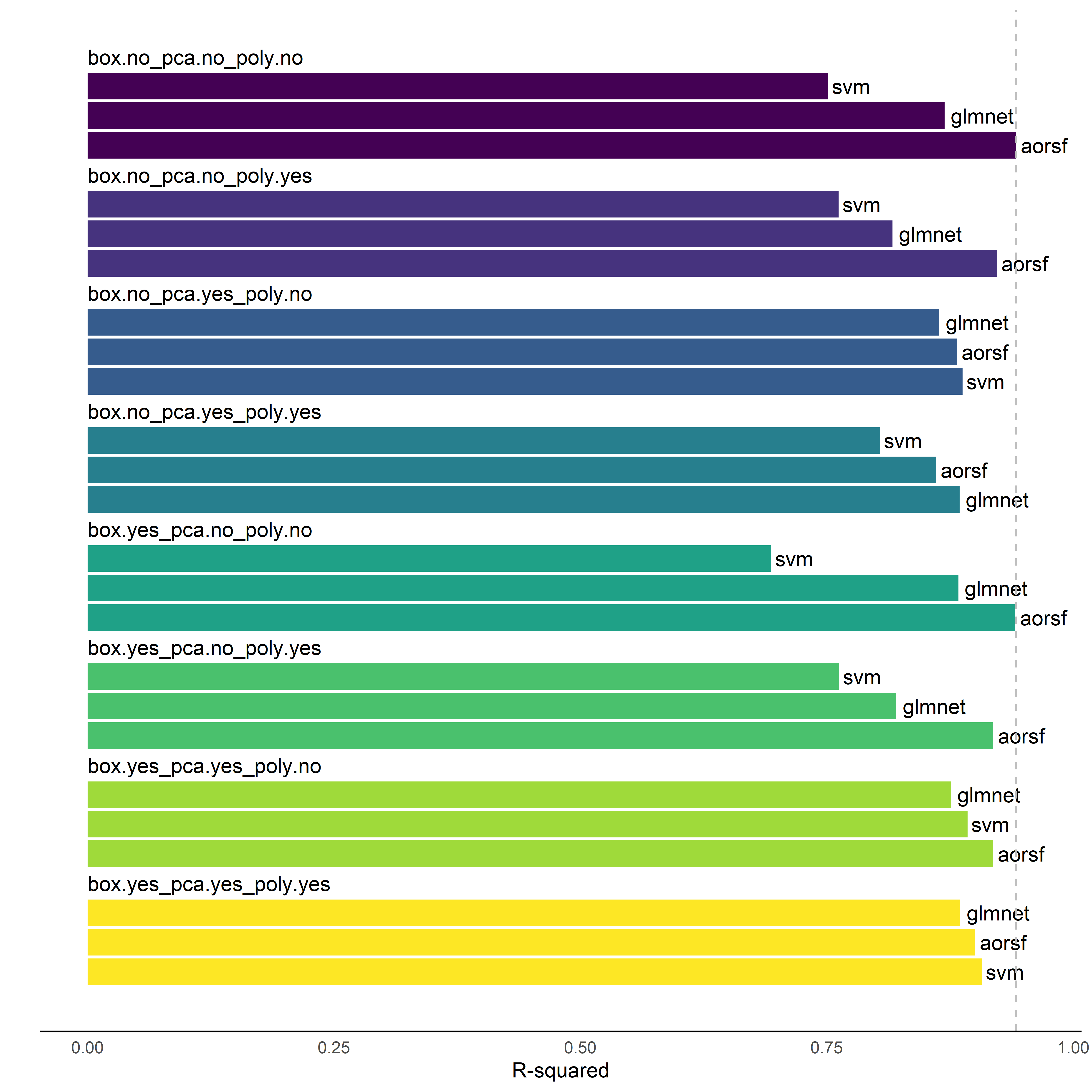
From the figure, we see
aorsfobtained the best overall prediction accuracy (i.e., \(R^2\) statistic in testing data) when it was given the plain, no extra step recipe. Thanks,aorsf, for making my experiment boring.the
svmlearner had very different prediction accuracy across recipes, and it even beat theaorsflearner in some recipes where principal component analysis was applied to numeric predictors.glmnetdoes pretty well everywhere, but it seems like using polynomials is only beneficial forglmnetif we also use principal component analysis.
Tabulate
In case you prefer looking at results grouped by model instead of grouped by recipe, here’s a little table that does so:
data_rsq <- wf_done %>%
 collect_metrics(summarize = TRUE) %>%
 separate(wflow_id,
          into = c("box", "pca", "poly", "model"),
          sep = '_') %>%
 mutate(
  poly = str_remove(poly, "\\.$"),
  across(c(box, pca, poly), ~ str_remove(.x, ".*\\."))
 ) %>%
 filter(.metric == 'rsq') %>%
 group_by(box, pca, poly, model) %>%
 arrange(desc(mean)) %>%
 slice(1) %>%
 select(box:model, mean, std_err) %>%
 arrange(model, desc(mean))

library(gt)

gt(data_rsq, groupname_col = 'model') %>%
 tab_options(table.width = pct(80)) %>%
 tab_spanner(label = "Pre-processing options",
             columns = c("box", "pca", "poly")) %>%
 tab_spanner(label = "Prediction accuracy",
             columns = c("mean", "std_err")) %>%
 cols_align('center') %>%
 cols_align('left', columns = 'box') %>%
 cols_label(box = "Box-cox",
            pca = "Principal components",
            poly = "Polynomials",
            mean = "R-squared",
std_err = "Standard error")| Pre-processing options | Prediction accuracy | |||
|---|---|---|---|---|
| Box-cox | Principal components | Polynomials | R-squared | Standard error |
| aorsf | ||||
| no | no | no | 0.9419690 | 0.009308679 |
| yes | no | no | 0.9413249 | 0.009697220 |
| no | no | yes | 0.9224564 | 0.014067223 |
| yes | no | yes | 0.9189269 | 0.013127552 |
| yes | yes | no | 0.9186974 | 0.009955760 |
| yes | yes | yes | 0.9003848 | 0.013711507 |
| no | yes | no | 0.8820053 | 0.015680558 |
| no | yes | yes | 0.8608096 | 0.028205456 |
| glmnet | ||||
| yes | yes | yes | 0.8854123 | 0.015113051 |
| no | yes | yes | 0.8846210 | 0.020529055 |
| yes | no | no | 0.8834284 | 0.012616637 |
| yes | yes | no | 0.8759954 | 0.016490965 |
| no | no | no | 0.8693738 | 0.023352998 |
| no | yes | no | 0.8641152 | 0.023903995 |
| yes | no | yes | 0.8206020 | 0.020318719 |
| no | no | yes | 0.8166270 | 0.025821975 |
| svm | ||||
| yes | yes | yes | 0.9074204 | 0.015053010 |
| yes | yes | no | 0.8926469 | 0.027590826 |
| no | yes | no | 0.8876902 | 0.024842583 |
| no | yes | yes | 0.8039769 | 0.029382297 |
| yes | no | yes | 0.7624643 | 0.048258825 |
| no | no | yes | 0.7619207 | 0.057404793 |
| no | no | no | 0.7514309 | 0.051145069 |
| yes | no | no | 0.6936020 | 0.043528774 |
Wrapping up
Use mirai - it’s a game changer. It works well with tidymodels and I’m betting it works well with just about any task that can be organized in a list.